FluxQubit
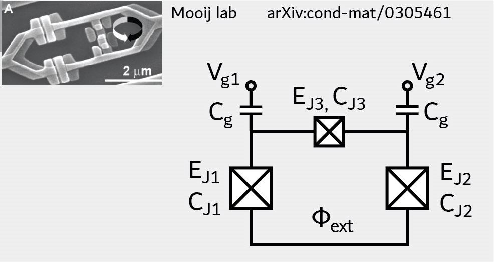
The flux qubit [Orlando1999] is described by the Hamiltonian
where \(i,j \in \{1,2\}, E_\text{C}=\tfrac{e^2}{2}C^{-1}\) and
\(C_{Ji}\) refers to the capacitance of the \(i^\text{th}\) junction and \(C_{gi}\) refers to the capacitance to ground of the \(i^\text{th}\) island. For simplicity, the Hamiltonian is written here in a mixed basis, however for the purposes of numerical diagonalization in the FluxQubit class, the charge basis is employed for both variables. The user must specify a charge-number cutoff ncut, chosen large enough so that convergence is achieved.
An instance of the flux qubit is initialized as follows:
EJ = 35.0
alpha = 0.6
fluxqubit = scqubits.FluxQubit(EJ1 = EJ,
                              EJ2 = EJ,
                              EJ3 = alpha*EJ,
                              ECJ1 = 1.0,
                              ECJ2 = 1.0,
                              ECJ3 = 1.0/alpha,
                              ECg1 = 50.0,
                              ECg2 = 50.0,
                              ng1 = 0.0,
                              ng2 = 0.0,
                              flux = 0.5,
                              ncut = 10)
From within Jupyter notebook, a flux qubit instance can alternatively be created with:
fluxqubit = scqubits.FluxQubit.create()
This functionality is enabled if the ipywidgets package is installed, and displays GUI forms prompting for
the entry of the required parameters.
Wavefunctions and visualization of eigenstates and the potential
|
Return a flux qubit wave function in phi1, phi2 basis |
|
Plots 2d phase-basis wave function. |
Draw contour plot of the potential energy. |
Implemented operators
The following operators are implemented for use in matrix element calculations.
|
Returns the charge number operator conjugate to \(\phi_1\) in the charge? or eigenenergy basis. |
|
Returns the charge number operator conjugate to \(\phi_2\) in the charge? or eigenenergy basis. |
Returns operator \(e^{i\phi_1}\) in the charge or eigenenergy basis. |
|
Returns operator \(e^{i\phi_2}\) in the charge or eigenenergy basis. |
|
Returns operator \(\cos \phi_1\) in the charge or eigenenergy basis. |
|
Returns operator \(\cos \phi_2\) in the charge or eigenenergy basis. |
|
Returns operator \(\sin \phi_1\) in the charge or eigenenergy basis. |
|
Returns operator \(\sin \phi_2\) in the charge or eigenenergy basis. |
Computation and visualization of matrix elements
|
Returns table of matrix elements for operator with respect to the eigenstates of the qubit. |
|
Plots matrix elements for operator, given as a string referring to a class method that returns an operator matrix. |
Calculates matrix elements for a varying system parameter, given an array of parameter values. |
|
Generates a simple plot of a set of eigenvalues as a function of one parameter. |
Estimation of coherence times
Show plots of coherence for various channels supported by the qubit as they vary as a function of a changing parameter. |
|
Plot effective \(T_1\) coherence time (rate) as a function of changing parameter. |
|
Plot effective \(T_2\) coherence time (rate) as a function of changing parameter. |
|
|
Calculate the transition time (or rate) using Fermi's Golden Rule due to a noise channel with a spectral density spectral_density and system noise operator noise_op. |
Calculate the effective \(T_1\) time (or rate). |
|
Calculate the effective \(T_2\) time (or rate). |
|
|
Calculate the 1/f dephasing time (or rate) due to arbitrary noise source. |
Calculate the 1/f dephasing time (or rate) due to critical-current noise from all three Josephson junctions \(EJ1\), \(EJ2\) and \(EJ3\). |