Eigenstate Labeling by Branch Analysis
Branch analysis is a scheme of labeling eigenstates of a joint quantum system by bare product state labels, described in [Dumas2024]. Besides its original purpose for understanding the dynamics during dispersive readout of a qubit, it is a systematic method to label eigenstates even for strongly interacting systems, where a simple “labeling by overlap” strategy is not applicable.
We demonstrate the branch analysis for a transmon-resonator system, defined as follows:
[3]:
# truncated dimension of the transmon and the resonator
N_tmon, N_res = 10, 50

tmon = scq.Transmon(
    EJ = 20,
    EC = 0.3,
    ng = 0.25,
    ncut = 100,
    truncated_dim = N_tmon,
)

res = scq.Oscillator(
    E_osc = 5,
    l_osc = 1,
    truncated_dim = N_res,
)

hilbertspace = scq.HilbertSpace([tmon, res])

hilbertspace.add_interaction(
    g = 0.1,
    op1 = tmon.n_operator,
    op2 = res.n_operator
)
Basic Procedure of Branch Analysis
Branch analysis associates the eigenstates with bare product state labels \((t, r)\), with \(t\) and \(r\) being the excitations in the transmon and resonator, respectively. It is performed in the following steps:
We begin with identifying an eigenstate of the system with the largest overlap with a bare product state \(|0,0\rangle\) and label it by \(|\overline{0,0}\rangle\).
For each bare label \((0, r)\), we find the corresponding eigenstate \(|\overline{0,r}\rangle\) recursively, starting from \(r=1\):
Put one resonator excitation on a labeled eigenstate \(|\overline{0,r-1}\rangle\), which yields a new state \(|\psi_e\rangle = a^\dagger |\overline{0,r-1}\rangle\);
Among all the unlabeled eigenstates, identify the eigenstate \(|\psi_g\rangle\) with the largest overlap with \(|\psi_e\rangle\);
Label \(|\psi_g\rangle\) by \(|\overline{0,r}\rangle\);
Repeat the steps a)—c) until \(r=N_\text{res}-1\), where \(N_\text{res}\) is the dimension of the truncated Hilbert space of the resonator mode. This procedure yields a set of eigenstates \(\{|\overline{0,r}\rangle\}_{n=0}^{N_\text{res}-1}\) corresponding to the transmon initialized in the ground state, and such set is called a branch.
To find other branches with different transmon excitations, we repeat the step 2 for different initial eigenstates \(|\overline{1, 0}\rangle\), \(|\overline{2, 0}\rangle\), etc. These initial eigenstates are found as follows:
Put one transmon excitation on a given labeled eigenstate \(|\overline{t-1,0}\rangle\). For a transmon (and any other non-linear modes), we define the excitation operator
\[T^+ = \sum_{t=1}^{N_\text{tmon}-1} |t\rangle\langle t-1| \otimes I_\text{res},\]where \(N_\text{tmon}\) is the dimension of the transmon’s Hilbert space. The corresponding excited state is given by \(|\psi_e\rangle = T^+ |\overline{t-1,0}\rangle\);
Among all the unlabeled eigenstates, identify the eigenstate \(|\psi_g\rangle\) with the largest overlap with \(|\psi_e\rangle\), which is labeled as \(|\overline{t,0}\rangle\).
The following figure summarizes the procedure for performing branch analysis for a system with \(N_\text{tmon}=3\) and \(N_\text{res}=4\): the numbers in front of each eigenstate show the order in which these states are labeled, and each arrow indicates how a labeled eigenstate is excited to help identify and label the next eigenstate.
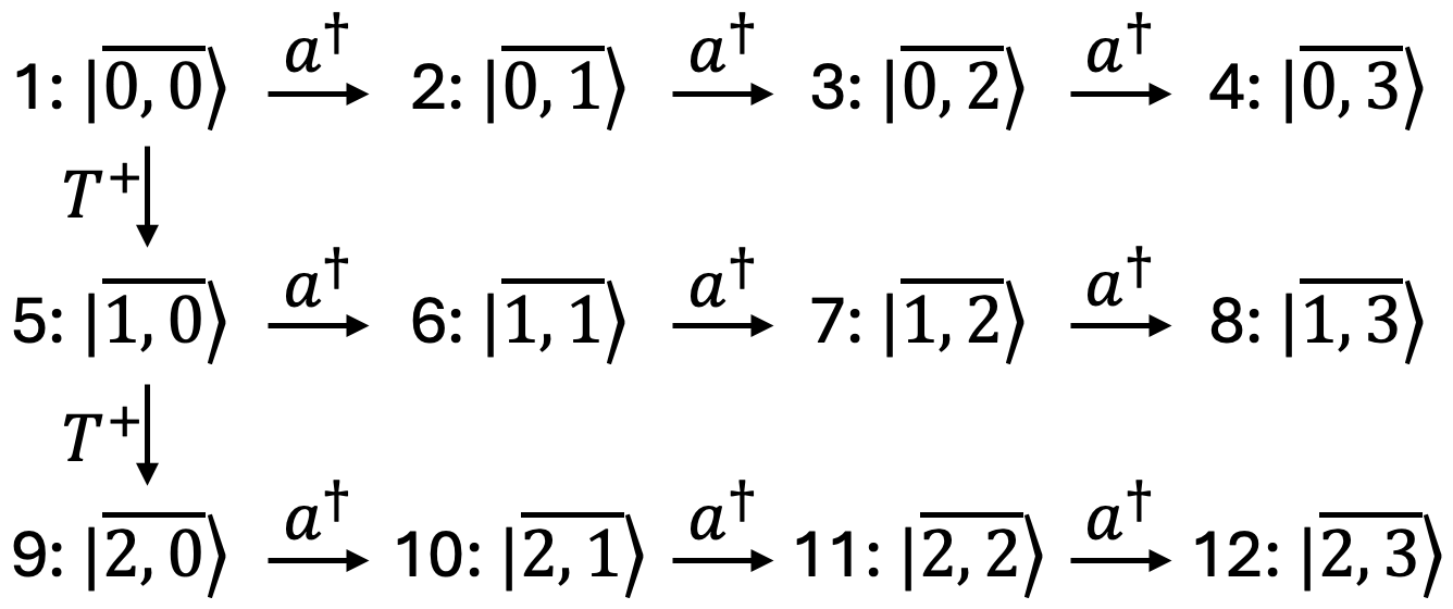
From the above figure, it is clear that the eigenstates are labeled in the lexical order of the bare product labels—the latter index \(r\) increases “faster” than the first index \(t\) in the iteration, just like the order of the words in a dictionary.
In the package, branch analysis can be performed as an option of the generate_lookup() function:
[3]:
hilbertspace.generate_lookup(
    ordering = 'LX'
)
The labeling of an eigenstate can be accessed by lookup functions described in section “Spectrum lookup: converting between bare and dressed indices” on page Composite Hilbert Spaces & QuTiP. For example, the \(8^{\text{th}}\) eigenstate is corresponding to the following bare product label:
[4]:
hilbertspace.bare_index(8)
[4]:
(2, 1)
Iteration with Specific Ordering
The above demonstration of branch analysis is based on the case where the resonator is the second subsystem, and the iteration over the bare labels naturally follows the lexical order.
However, this is not the case if the resonator is the first subsystem, i.e., the joint system is defined by
hilbertspace = HilbertSpace([res, tmon])
To perform the desired branch analysis, we need to manually specify the subsys_priority in the generate_lookup() function, which defines a permutation of the bare labels
hilbertspace.generate_lookup(
    ordering = 'LX',
    subsys_priority = [1, 0]
)
Branch analysis will be performed according to lexical ordering of the permuted labels, which can be summarized in the following figure:
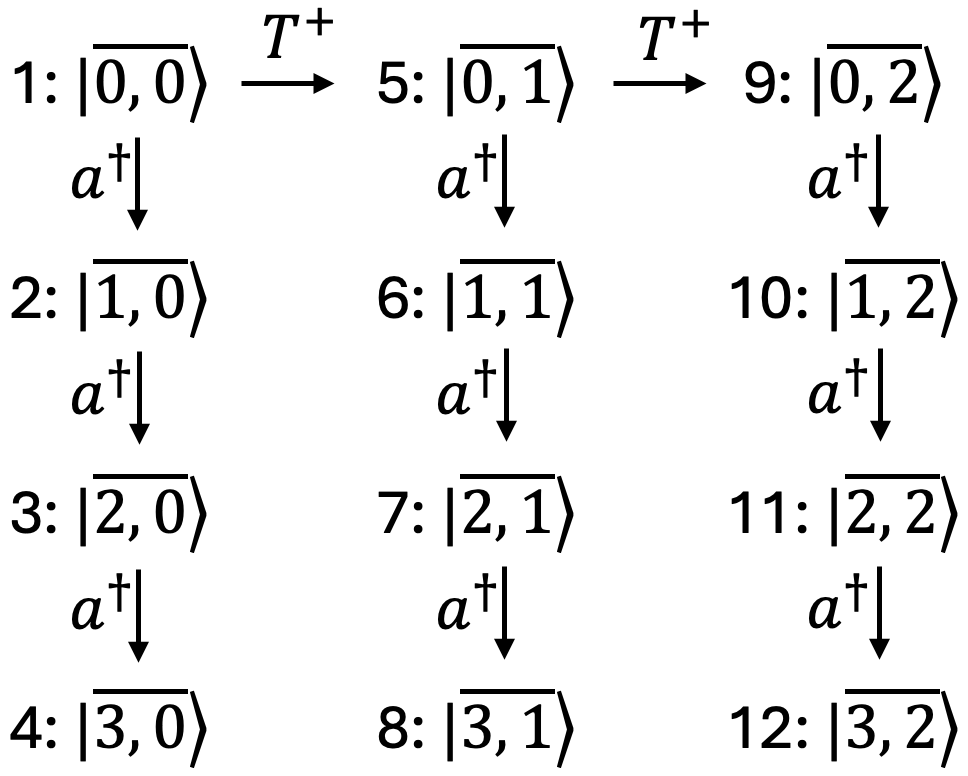
By default, we do not permute the bare labels, i.e., subsys_priority is set to [0, 1, ..., s-1], where \(s\) is the number of subsystems.
Label a Partial Set of Eigentates
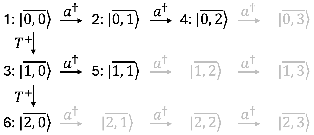
Performing branch analysis for a high-dimensional system can be time consuming, which may even be slower than diagonalizing the Hamiltonian. In some cases, one may be interested in the low-energy states and only want to label a partial set of eigenstates to save time. This can be done in a similar spirit of the branch analysis as follows.
As an example, we label the eigenstates corresponding to the six lowest-energy bare product states. For a bare product state \(|t, r\rangle\), we compute its energy before two subsystems are coupled
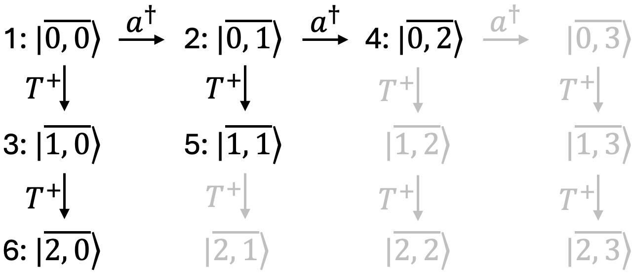
where \(E^\text{tmon}_t\) and \(E^\text{res}_r\) are eigenenergies for the transmon and the resonator, respectively. Assume the energies of the lowest six bare product states are ordered as follows:
The labeling of the eigenstates can be described by the following figure, with unlabeled eigenstates in gray:
This is done by setting ordering='BE' (Bare Energy ordering)
[5]:
hilbertspace.generate_lookup(
    ordering = 'BE',
    BEs_count = 6
)
“BE” ordering can be tuned by subsys_priority argument, and this controls where to put the next excitation to label the next eigenstate. For example, with subsys_priority=[1, 0], the labeling follows follows the pattern shown in the figure. Different from the case using a default subsys_priority, the eigenstate labeled \((1,1)\) is identified by applying the transmon excitation operator to the previously labeled state \(|\overline{0,1}\rangle\).