Explorer

The Explorer helps visualize properties of coupled quantum systems and how they change when system parameters are varied. The Explorer provides an interactive display with multiple adjustable panels.

The workflow is to generate a HilbertSpace object specifying the physical system, and a ParameterSweep object that contains all data to be visualized. Once this data is stored, the Explorer class is invoked for display.

Example 1: fluxonium coupled to resonator

As a first example, we consider a system composed of a fluxonium qubit, coupled through its charge operator to the voltage inside a resonator.

HilbertSpace setup

The initialization of the composite Hilbert space proceeds as usual; we first define the individual two subsystems that will make up the Hilbert space:

import numpy as np
import scqubits as scq


qbt = scq.Fluxonium(
    EJ=2.55,
    EC=0.72,
    EL=0.12,
    flux=0.0,
    cutoff=110,
    truncated_dim=9
)

osc = scq.Oscillator(
    E_osc=7.4,
    truncated_dim=5
)

Here, the truncated_dim parameters are important. For the fluxonium, with cutoff set to 110, the internal Hilbert space dimension is 110. Once diagonalized, we will only keep a few eigenstates going forward - in the above example 9. Similarly, we keep 5 levels for the resonators, i.e., photon states n=0,1,…,4 are included in the following.

Next, the two subsystems are declared as the two components of a joint Hilbert space:

hilbertspace = scq.HilbertSpace([qbt, osc])

The interaction between fluxonium and resonator is of the form \(H_\text{int} = g n (a+a^\dagger)\), where \(n\) is the fluxonium’s charge operator: qbt.n_operator(). This structure is captured by creating an InteractionTerm object via add_interaction:

hilbertspace.add_interaction(
    g_strength=0.2,
    op1=qbt.n_operator,
    op2=osc.creation_operator,
    add_hc=True
)

Parameter sweep setup

We consider sweeping the external flux through the fluxonium loop. To create the necessary ParameterSweep object, we specify: 1. param_name: the name of the sweep parameter (below expressed in LaTeX format as the flux in units of the flux quantum) 2. param_vals_by_name: a dictionary that names our parameter and associates the array of flux values with it 3. subsys_update_info (optional): a dictionary listing the particular Hilbert space subsystems that change as each parameter (here the flux) is varied 4. update_hilbertspace(param_val): a function that shows how a change in the sweep parameter affects the Hilbert space; here only the .flux attributed of the fluxonium qubit needs to be changed

These ingredients all make it into the initialization of the ParameterSweep object. Once initialized, spectral data is generated and stored. Here, we additionally generate data for dispersive shifts and charge matrix elements.

param_name = "Φext/Φ0"
param_vals = np.linspace(0, 1.0, 101)


def update_hilbertspace(param_val):
    qbt.flux = param_val


sweep = scq.ParameterSweep(
    paramvals_by_name={param_name: param_vals},
    evals_count=10,
    hilbertspace=hilbertspace,
    subsys_update_info={param_name: [qbt]},
    update_hilbertspace=update_hilbertspace,
    num_cpus=4
)

Starting the Explorer class

At this point, everything is prepared to start the interactive Explorer display!

explorer = scq.Explorer(sweep)

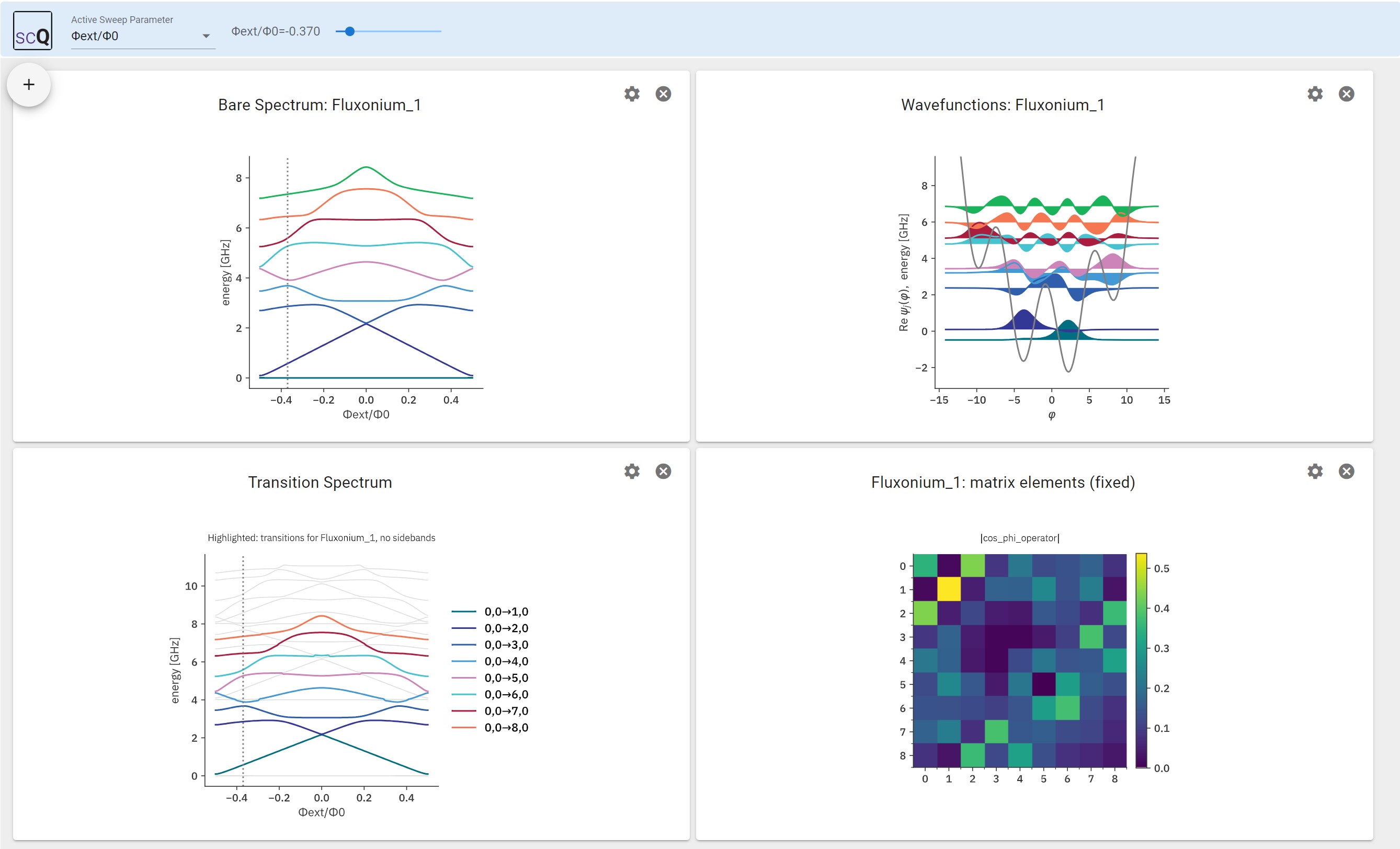
Note

Transition plots rely on the identification of bare product states with dressed states, based on a simple overlap criterion. Whenever qubit levels cross and hybridize with, e.g., a resonator, this identification cannot succeed, and plots will “drop out” in this region. (This is intended, not a bug.)

Example 2: two transmons coupled to a resonator

In the following second example, we consider a system composed of two flux-tunable transmons, capacitively coupled to one joint harmonic mode. (The flux is assumed to arise from a global field, and the SQUID-loop areas of the two transmons are different with an area ratio of 1.4)

Hilbert space setup

qbt1 = scq.Transmon(
     EJ=25.0,
     EC=0.2,
     ng=0,
     ncut=30,
     truncated_dim=3)

qbt2 = scq.Transmon(
     EJ=15.0,
     EC=0.15,
     ng=0,
     ncut=30,
     truncated_dim=3)


resonator = scq.Oscillator(
    E_osc=5.5,
    truncated_dim=4)

hilbertspace = scq.HilbertSpace([qbt1, qbt2, resonator])


g1 = 0.1  # coupling resonator-CPB1 (without charge matrix elements)
g2 = 0.2  # coupling resonator-CPB2 (without charge matrix elements)

hilbertspace.add_interaction(
    g_strength = g1,
    op1 = qbt1.n_operator,
    op2 = resonator.creation_operator,
    add_hc = True
)

hilbertspace.add_interaction(
    g_strength = g2,
    op1 = qbt2.n_operator,
    op2 = resonator.creation_operator,
    add_hc = True
)

Parameter sweep setup

param_name = "Φext/Φ0"
param_vals = np.linspace(0.0, 1.0, 151)

subsys_update_list = [qbt1, qbt2]


def update_hilbertspace(param_val):     # function that shows how Hilbert space components are updated
    qbt1.EJ = 30*np.abs(np.cos(np.pi * param_val))
    qbt2.EJ = 40*np.abs(np.cos(np.pi * param_val * 2))


sweep = scq.ParameterSweep(
    paramvals_by_name={param_name: param_vals},
    evals_count=15,
    hilbertspace=hilbertspace,
    subsys_update_info={param_name: [qbt1, qbt2]},
    update_hilbertspace=update_hilbertspace,
)

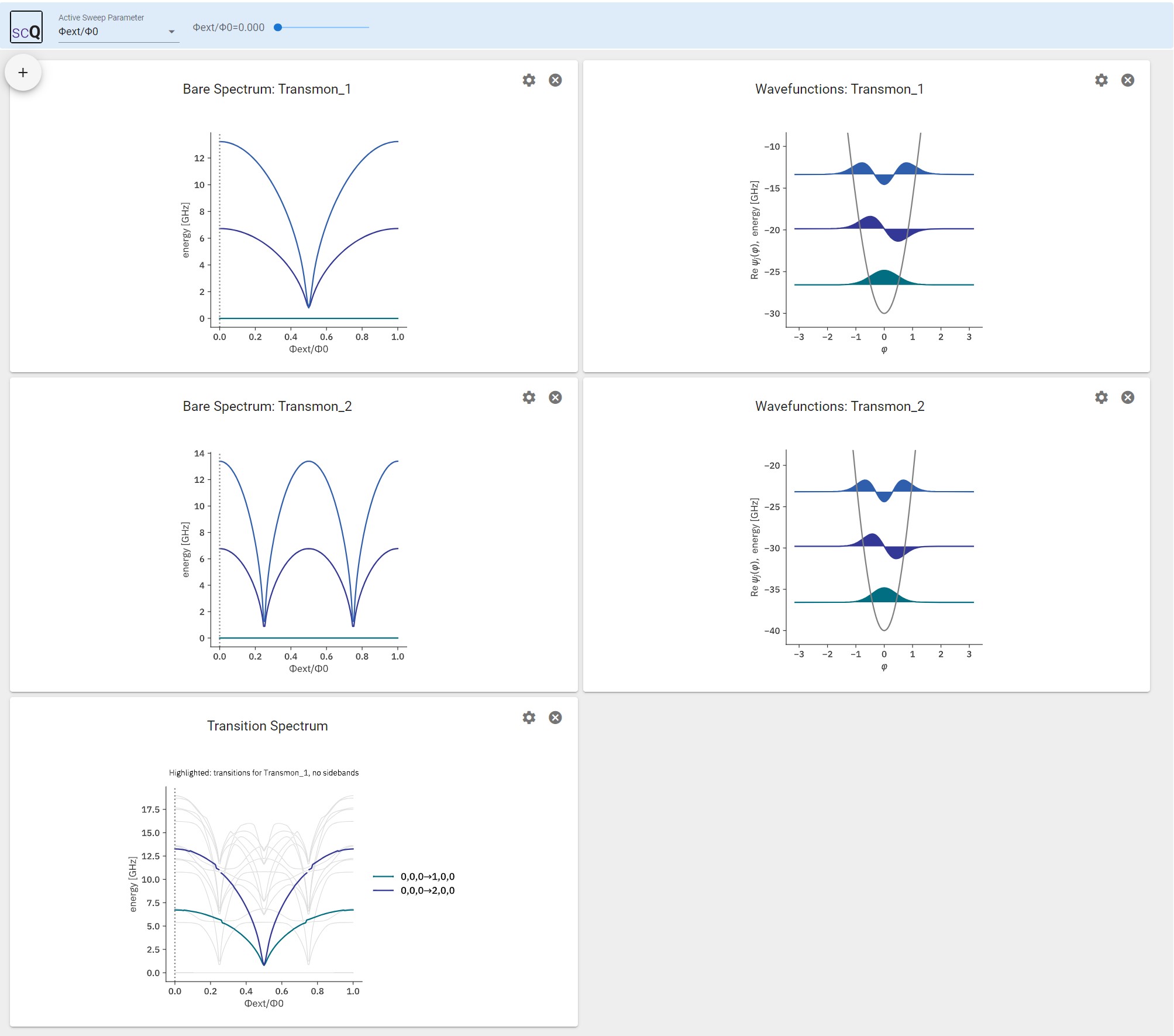
Start Explorer

explorer = scq.Explorer(sweep=sweep)