Composite Hilbert Spaces & QuTiP#

The HilbertSpace class provides data structures and methods for handling composite Hilbert spaces which may consist of multiple qubits and/or oscillators coupled to each other. To harness the power of QuTiP (a toolbox for simulating stationary and dynamical properties of closed and open quantum systems), HilbertSpace provides a convenient interface: it generates qutip.qobj objects which can then be handed over directly to QuTiP.

In the following, the basic functionality of the HilbertSpace class is illustrated for the example of two transmons coupled to a harmonic mode.

Transmon qubits can be capacitively coupled to a common harmonic mode, realized by an LC oscillator or a transmission-line resonator. The Hamiltonian describing such a composite system is given by: \begin{equation} H=H_\text{tmon,1} + H_\text{tmon,2} + \omega_r a^\dagger a + \sum_{j=1,2}g_j n_j(a+a^\dagger), \end{equation} where \(j=1,2\) enumerates the two transmon qubits, \(\omega_r\) is the (angular) frequency of the resonator. Furthermore, \(n_j\) is the charge number operator for qubit \(j\), and \(g_j\) is the coupling strength between qubit \(j\) and the resonator.

Creating a HilbertSpace instance#

The first step consists of creating the objects describing the individual building blocks of the full Hilbert space. Here, these will be the two transmons and one oscillator:

[2]:

tmon1 = scq.Transmon(
    EJ=40.0,
    EC=0.2,
    ng=0.3,
    ncut=40,
    truncated_dim=4     # after diagonalization, we will keep levels 0, 1, 2, and 3
)

tmon2 = scq.Transmon(
    EJ=15.0,
    EC=0.15,
    ng=0.0,
    ncut=30,
    truncated_dim=4
)

resonator = scq.Oscillator(
    E_osc=4.5,
    truncated_dim=4  # up to 3 photons (0,1,2,3)
)

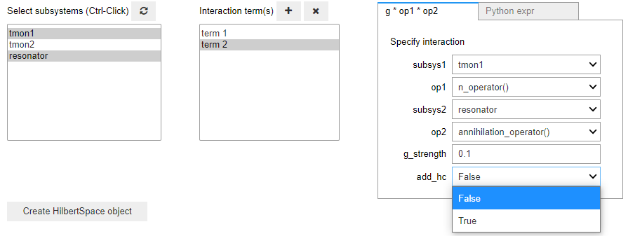
The HilbertSpace object is now created in one of two ways. The first is by utilizing the GUI:

[3]:

g = 0.1
hilbertspace = scq.HilbertSpace.create()

title

The second way of creating a HilbertSpace object is through regular programmatic creation: provide a list of all subsystems and then specify individual interaction terms (see the next subsection for the latter):

[4]:

hilbertspace = scq.HilbertSpace([tmon1, tmon2, resonator])
print(hilbertspace)

HilbertSpace:  subsystems
-------------------------

Transmon------------| [Transmon_1]
                    | EJ: 40.0
                    | EC: 0.2
                    | ng: 0.3
                    | ncut: 40
                    | truncated_dim: 4
                    |
                    | dim: 81


Transmon------------| [Transmon_2]
                    | EJ: 15.0
                    | EC: 0.15
                    | ng: 0.0
                    | ncut: 30
                    | truncated_dim: 4
                    |
                    | dim: 61


Oscillator----------| [Oscillator_1]
                    | E_osc: 4.5
                    | l_osc: None
                    | truncated_dim: 4
                    |
                    | dim: 4

Specifying interactions between subsystems#

Interaction terms describing the coupling between subsystems can be specified in three different ways.

Option 1: operator-product based interface#

Interaction terms involving multiple subsystems \(S=1,2,3,\ldots\) are often of the form

\(V = g A_1 A_2 A_3 \cdots \qquad \text{or} \qquad V = g B_1 B_2 B_3 \cdots + \text{h.c.}\)

where the operators \(A_j\), \(B_j\) act on subsystem \(j\). In the first case, the operators \(A_j\) are expected to be hermitean.

This structure is captured by using the add_interaction method in the following way:

[5]:

g1 = 0.1  # coupling resonator-tmon1 (without charge matrix elements)
operator1 = tmon1.n_operator()
operator2 = resonator.creation_operator() + resonator.annihilation_operator()

hilbertspace.add_interaction(
    g=g1,
    op1=(operator1, tmon1),
    op2=(operator2, resonator)
)

g2 = 0.2  # coupling resonator-CPB2 (without charge matrix elements)
hilbertspace.add_interaction(
    g=g2,
    op1=tmon2.n_operator,
    op2=resonator.creation_operator,
    add_hc=True
)

In this instance, op1 and op2 take either

(<array>, <subsystem>): a tuple with an array or sparse matrix in the first position and the subsystem in the second position, or
<callable>: the operator as a callable function (which will automatically yield the subsystem the operator function is bound to).

These two choices can be mixed and matched.

Note:

Interactions based on only one operator are enabled (simply drop the op2 entry). One use case of this is to create a higher order non-linearity \(a^\dagger a^\dagger a^\dagger a a a\) in a Kerr oscillator.
Interactions with more than two operators are built by specifying op3, op4, etc.

The option add_hc = True adds the hermitian conjugate to the Hamiltonian, and is available in the present operator-product based interface, as well as in the one described next as option 2.

Option 2: string- based interface#

The add_interaction method can also be used to define the interaction in string form, providing an expression that can be evaluated by the Python interpreter (after operator name substitution).

[6]:

hilbertspace_example = scq.HilbertSpace([tmon1, tmon2, resonator])

g3 = 0.1

hilbertspace_example.add_interaction(
    expr="g3 * cos(n) * adag",
    op1=("n", tmon1.n_operator),
    op2=("adag", resonator.creation_operator),
    add_hc=True
)

expr is a string used to define the interaction as a Python expression. It should use variables that are already defined globally, and operators given by the names provided in op1, op2, op3, etc. When using expr, each argument op1, op2, … should be a tuple of the form (<operator name as string>, <operator as callable>) or (<operator name as string>, <operator as array | sparse matrix>, <subsystem>).

Beyond built-in Python functions and operations, acceptable functions to use in expr are:

Function	Function translation
`'cos'`	`'Qobj.cosm'`
`'sin'`	`'Qobj.sinm'`
`'exp'`	`'Qobj.expm'`
`'sqrt'`	`'Qobj.sqrtm'`

Option 3: Qobj interface#

Finally add_interaction can also been used to directly add a Qobj object that has already been properly identity wrapped:

[7]:

# Generate a Qobj
g = 0.1
a = qt.destroy(4)
kerr = a.dag() * a.dag() * a * a
id = qt.qeye(4)
V = g * qt.tensor(id, id, kerr)

hilbertspace_example.add_interaction(qobj = V)

In this case, the add_interaction method only requires the argument qobj which must be an object of the type Qobj.

Obtaining the Hamiltonian#

With the interactions specified, the full Hamiltonian of the coupled system can be obtained via the method .hamiltonian(). This conveniently results in a qubit.Qobj operator:

[8]:

dressed_hamiltonian = hilbertspace.hamiltonian()
dressed_hamiltonian

[8]:

Quantum object: dims = [[4, 4, 4], [4, 4, 4]], shape = (64, 64), type = oper, isherm = True\begin{equation*}\left(\begin{array}{*{11}c}-48.968 & 0.030 & 0.0 & 0.0 & 0.0 & \cdots & 0.0 & 0.0 & 0.0 & 0.0 & 0.0\\0.030 & -44.468 & 0.042 & 0.0 & 0.261 & \cdots & 0.0 & 0.0 & 0.0 & 0.0 & 0.0\\0.0 & 0.042 & -39.968 & 0.052 & 0.0 & \cdots & 0.0 & 0.0 & 0.0 & 0.0 & 0.0\\0.0 & 0.0 & 0.052 & -35.468 & 0.0 & \cdots & 0.0 & 0.0 & 0.0 & 0.0 & 0.0\\0.0 & 0.261 & 0.0 & 0.0 & -44.881 & \cdots & 0.0 & 0.0 & 0.0 & 0.0 & 0.0\\\vdots & \vdots & \vdots & \vdots & \vdots & \ddots & \vdots & \vdots & \vdots & \vdots & \vdots\\0.0 & 0.0 & 0.0 & 0.0 & 0.0 & \cdots & -4.723 & 0.0 & 0.0 & -0.749 & 0.0\\0.0 & 0.0 & 0.0 & 0.0 & 0.0 & \cdots & 0.0 & -14.477 & 0.030 & 0.0 & 0.0\\0.0 & 0.0 & 0.0 & 0.0 & 0.0 & \cdots & 0.0 & 0.030 & -9.977 & 0.042 & 0.0\\0.0 & 0.0 & 0.0 & 0.0 & 0.0 & \cdots & -0.749 & 0.0 & 0.042 & -5.477 & 0.052\\0.0 & 0.0 & 0.0 & 0.0 & 0.0 & \cdots & 0.0 & 0.0 & 0.0 & 0.052 & -0.977\\\end{array}\right)\end{equation*}

This matrix is the representation of the Hamiltonian in the bare product basis.

The non-interacting (“bare”) Hamiltonian and the interaction Hamiltonian can be accessed similarly by using the methods .bare_hamiltonian() and .interaction_hamiltonian().

Obtaining the eigenspectrum via QuTiP#

Since the Hamiltonian obtained this way is a proper qutip.qobj, all QuTiP routines are now available. In the first case, we are still making use of the scqubit HilbertSpace.eigensys() method. In the second, case, we use QuTiP’s method .eigenenergies():

[9]:

evals, evecs = hilbertspace.eigensys(evals_count=4)
print(evals)

[-48.97770317 -45.02707241 -44.36656205 -41.18438832]

[10]:

dressed_hamiltonian = hilbertspace.hamiltonian()
dressed_hamiltonian.eigenenergies()

[10]:

array([-48.97770317, -45.02707241, -44.36656205, -41.18438832,
       -41.1776098 , -40.46448065, -39.76202396, -37.45533167,
       -37.22705488, -36.65156212, -36.56694139, -35.88617024,
       -35.14255357, -33.58960343, -33.38439485, -33.12061816,
       -32.66494366, -32.04065582, -31.96284558, -30.93536847,
       -29.65538466, -29.63912664, -28.97946785, -28.85287223,
       -28.64748897, -28.09427075, -27.35745603, -26.97461415,
       -26.21586637, -25.79648462, -25.3216198 , -25.07747135,
       -24.37567532, -24.24760531, -23.66618527, -23.15199748,
       -22.2580349 , -22.06752989, -21.57303944, -21.26626732,
       -20.85288717, -20.51511596, -19.78521899, -19.1938092 ,
       -18.41228666, -17.73463904, -17.66080329, -16.93618597,
       -16.66699841, -15.89010361, -15.58181323, -14.68288545,
       -13.84725844, -13.27037775, -13.08388811, -12.34366698,
       -11.62655644, -10.308913  ,  -9.23168892,  -8.32791939,
        -8.13883089,  -5.82301882,  -4.18180351,  -0.88957289])

Spectrum lookup: converting between bare and dressed indices#

We can refer to eigenstates and eigenenergies of the interacting quantum systems in two ways:

dressed indices: enumerating eigenenergies and -states as j=0,1,2,... starting from the ground state
bare product state indices: for a Hilbert space composed of three subsystems, specify tuples of the form (l,m,n) where l, m, n denote the excitation levels of each bare subsystem.

To use lookup functions converting back and forth between these indexing schemes, first generate the spectrum lookup table via:

[11]:

hilbertspace.generate_lookup()

This makes lookup functions available via hilbertspace.lookup.<lookup method> where

lookup method	purpose
`bare_index`	yields bare product state index for given dressed index
`dressed_index`	yields dressed index for given bare product state index

`energy_dressed_index`	return eigenenergy for given dressed index
`energy_bare_index`	return eigenenergy for given bare product-state index

`bare_eigenenergies`	return bare eigenenergies for specified subsystem
`bare_eigenstates`	return bare eigenstates for specified subsystem
`bare_productstate`	return bare product state for given bare index

Here are the bare energies of the first Cooper pair box system:

[12]:

tmon1_idx = hilbertspace.get_subsys_index(tmon1)
hilbertspace["bare_evals"][tmon1_idx]

[12]:

NamedSlotsNdarray([[-36.05064983, -28.25601136, -20.67410141,
                    -13.31487799]])

The dressed state with index j=8 corresponds to following bare product state index:

[13]:

hilbertspace.bare_index(8)

[13]:

(1, 1, 0)

The bare product state (2,1,0) most closely matches the following dressed state:

[14]:

hilbertspace.dressed_index((2, 1, 0))

[14]:

This is the eigenenergy for dressed index j=10:

[15]:

hilbertspace.energy_by_dressed_index(10)

[15]:

-36.56694138527016

Helper function: identity wrapping#

The abbreviated notation commonplace in physics usually omits tensor products with identities. As an example, in a composite Hilbert space consisting of three subsystems \(j=1,2,3\) with individual Hamiltonians \(H_j\), we typically use the notation

\(H=H_1+H_2+H_3\)

which is meant to stand for

\(H = H_1\otimes\mathbb{I}\otimes \mathbb{I} + \mathbb{I}\otimes H_2\otimes \mathbb{I} + \mathbb{I}\otimes\mathbb{I}\otimes H_3\)

In most places of the HilbertSpace class, scqubits manages this “identity wrapping” automatically. In some use cases, it may become necessary to invoke this functionality manually. For that purpose, scqubits implements the helper routine identity_wrap. For instance, the term \(\mathbb{I}\otimes H_2\otimes \mathbb{I}\) would be generated via the pseudocode scq.identity_wrap(H2, subsystem2, [subsystem1, subsystem2, subsystem3]).

In the context of the above example of two transmons coupled to an oscillator, the identity-wrapped charge operator of the second transmon is generated via

[21]:

scq.identity_wrap(tmon2.n_operator(), tmon2, hilbertspace.subsystem_list)

[21]:

Quantum object: dims = [[4, 4, 4], [4, 4, 4]], shape = (64, 64), type = oper, isherm = True\begin{equation*}\left(\begin{array}{*{11}c}0.0 & 0.0 & 0.0 & 0.0 & 1.305 & \cdots & 0.0 & 0.0 & 0.0 & 0.0 & 0.0\\0.0 & 0.0 & 0.0 & 0.0 & 0.0 & \cdots & 0.0 & 0.0 & 0.0 & 0.0 & 0.0\\0.0 & 0.0 & 0.0 & 0.0 & 0.0 & \cdots & 0.0 & 0.0 & 0.0 & 0.0 & 0.0\\0.0 & 0.0 & 0.0 & 0.0 & 0.0 & \cdots & 0.0 & 0.0 & 0.0 & 0.0 & 0.0\\1.305 & 0.0 & 0.0 & 0.0 & 0.0 & \cdots & 0.0 & 0.0 & 0.0 & 0.0 & 0.0\\\vdots & \vdots & \vdots & \vdots & \vdots & \ddots & \vdots & \vdots & \vdots & \vdots & \vdots\\0.0 & 0.0 & 0.0 & 0.0 & 0.0 & \cdots & 0.0 & 0.0 & 0.0 & 0.0 & -2.162\\0.0 & 0.0 & 0.0 & 0.0 & 0.0 & \cdots & 0.0 & 0.0 & 0.0 & 0.0 & 0.0\\0.0 & 0.0 & 0.0 & 0.0 & 0.0 & \cdots & 0.0 & 0.0 & 0.0 & 0.0 & 0.0\\0.0 & 0.0 & 0.0 & 0.0 & 0.0 & \cdots & 0.0 & 0.0 & 0.0 & 0.0 & 0.0\\0.0 & 0.0 & 0.0 & 0.0 & 0.0 & \cdots & -2.162 & 0.0 & 0.0 & 0.0 & 0.0\\\end{array}\right)\end{equation*}

The complete interface is:

scq.identity_wrap(operator, subsystem, subsys_list, op_in_eigenbasis=False, evecs=None)

Wrap given operator in subspace subsystem in identity operators to form full Hilbert-space operator.

Parameters

operator: operator acting in Hilbert space of subsystem; if str, then this should be an operator name in the subsystem, typically not in eigenbasis
subsystem (QuantumSys): subsystem to which operator belongs
subsys_list: list of all subsystems (in fixed order!)
op_in_eigenbasis (bool, optional): whether operator is given in the subsystem eigenbasis; otherwise, the internal QuantumSys basis is assumed
evecs (ndarray, optional): internal QuantumSys eigenstates, used to convert operator into eigenbasis

Return type: Qobj

Helper function: subsystem operator in dressed basis#

Oftentimes for qutip simulations, the most natural basis to use is the dressed basis of the full system. This way, any transitions between basis states are the result of additional (usually time-dependent) drives. These drives are often given in terms of an operator of one of the subsystems. We would like to transform that operator into the dressed basis. This requires two transformations: the first is from the “native” basis of the subsystem (for instance the charge basis for the transmon) into its bare eigenbasis, which is the basis used in HilbertSpace. The second is from the bare eigenbasis into the dressed eigenbasis.

For instance, the charge operator of the first transmon system may be expressed in the dressed eigenbasis as

[16]:

hilbertspace.op_in_dressed_eigenbasis(op=tmon1.n_operator)

[16]:

Quantum object: dims = [[4, 4, 4], [4, 4, 4]], shape = (64, 64), type = oper, isherm = True\begin{equation*}\left(\begin{array}{*{11}c}0.301 & -0.039 & -0.085 & -8.168\times10^{-06} & 1.558 & \cdots & -1.122\times10^{-10} & 1.605\times10^{-10} & -9.217\times10^{-11} & 7.380\times10^{-11} & -1.485\times10^{-10}\\-0.039 & 0.301 & -9.554\times10^{-08} & 0.047 & 2.549\times10^{-07} & \cdots & 1.951\times10^{-08} & 8.473\times10^{-09} & 1.147\times10^{-08} & -1.311\times10^{-08} & 2.163\times10^{-10}\\-0.085 & -9.554\times10^{-08} & 0.301 & -0.002 & 1.847\times10^{-08} & \cdots & 2.048\times10^{-08} & 2.181\times10^{-08} & 2.198\times10^{-08} & -2.874\times10^{-08} & 2.137\times10^{-11}\\-8.168\times10^{-06} & 0.047 & -0.002 & 0.301 & 3.679\times10^{-07} & \cdots & 6.351\times10^{-08} & 2.604\times10^{-06} & 2.402\times10^{-08} & -1.360\times10^{-08} & 2.820\times10^{-08}\\1.558 & 2.549\times10^{-07} & 1.847\times10^{-08} & 3.679\times10^{-07} & 0.301 & \cdots & -1.520\times10^{-10} & -5.187\times10^{-09} & -5.495\times10^{-09} & 9.614\times10^{-09} & -7.209\times10^{-11}\\\vdots & \vdots & \vdots & \vdots & \vdots & \ddots & \vdots & \vdots & \vdots & \vdots & \vdots\\-1.122\times10^{-10} & 1.951\times10^{-08} & 2.048\times10^{-08} & 6.351\times10^{-08} & -1.520\times10^{-10} & \cdots & 0.298 & 0.006 & -7.660\times10^{-05} & -0.002 & -2.577\\1.605\times10^{-10} & 8.473\times10^{-09} & 2.181\times10^{-08} & 2.604\times10^{-06} & -5.187\times10^{-09} & \cdots & 0.006 & 0.302 & 0.083 & -0.277 & 0.021\\-9.217\times10^{-11} & 1.147\times10^{-08} & 2.198\times10^{-08} & 2.402\times10^{-08} & -5.495\times10^{-09} & \cdots & -7.660\times10^{-05} & 0.083 & 0.302 & -0.006 & -0.461\\7.380\times10^{-11} & -1.311\times10^{-08} & -2.874\times10^{-08} & -1.360\times10^{-08} & 9.614\times10^{-09} & \cdots & -0.002 & -0.277 & -0.006 & 0.303 & -0.248\\-1.485\times10^{-10} & 2.163\times10^{-10} & 2.137\times10^{-11} & 2.820\times10^{-08} & -7.209\times10^{-11} & \cdots & -2.577 & 0.021 & -0.461 & -0.248 & 0.308\\\end{array}\right)\end{equation*}

Alternatively, the function may be called by supplying both a pair (<operator as ndarray>, <subsys>), as well as information on if the subsystem operator is already expressed in the bare eigenbasis. Examples of both cases (subsystem operator expressed in the native and bare eigenbasis) follow:

[19]:

hilbertspace.op_in_dressed_eigenbasis(op=(tmon1.n_operator(), tmon1), op_in_bare_eigenbasis=False)

[19]:

[20]:

n_1_bare_eigenbasis = tmon1.n_operator(energy_esys=True)
hilbertspace.op_in_dressed_eigenbasis(op=(n_1_bare_eigenbasis, tmon1), op_in_bare_eigenbasis=True)

[20]:

There are thus two interfaces for this operator: the first is

hilbertspace.op_in_dressed_eigenbasis(op=op)

Parameters

op (callable): operator acting in Hilbert space of subsystem

The second interface is

hilbertspace.op_in_dressed_eigenbasis(op=(op, subsys), op_in_bare_eigenbasis=False)

Parameters

op (ndarray, QuantumSys): pair of operator as ndarray as well as the subsystem to which the operator belongs
op_in_bare_eigenbasis (bool, optional): whether operator is given in the subsystem eigenbasis; otherwise, the internal QuantumSys basis is assumed

Return type: Qobj

The phases of the matrix elements of the operator in the dressed basis will depend on the phases of the dressed eigenvectors. To standardize those phases, scqubits also provides a helper function hilbertspace.standardize_eigenvector_phases() which standardizes the phases of the precalculated dressed eigenvectors. This function takes no arguments and returns nothing. It can be called before calling op_in_dressed_eigenbasis:

[ ]:

hilbertspace.standardize_eigenvector_phases()