Cos2PhiQubit

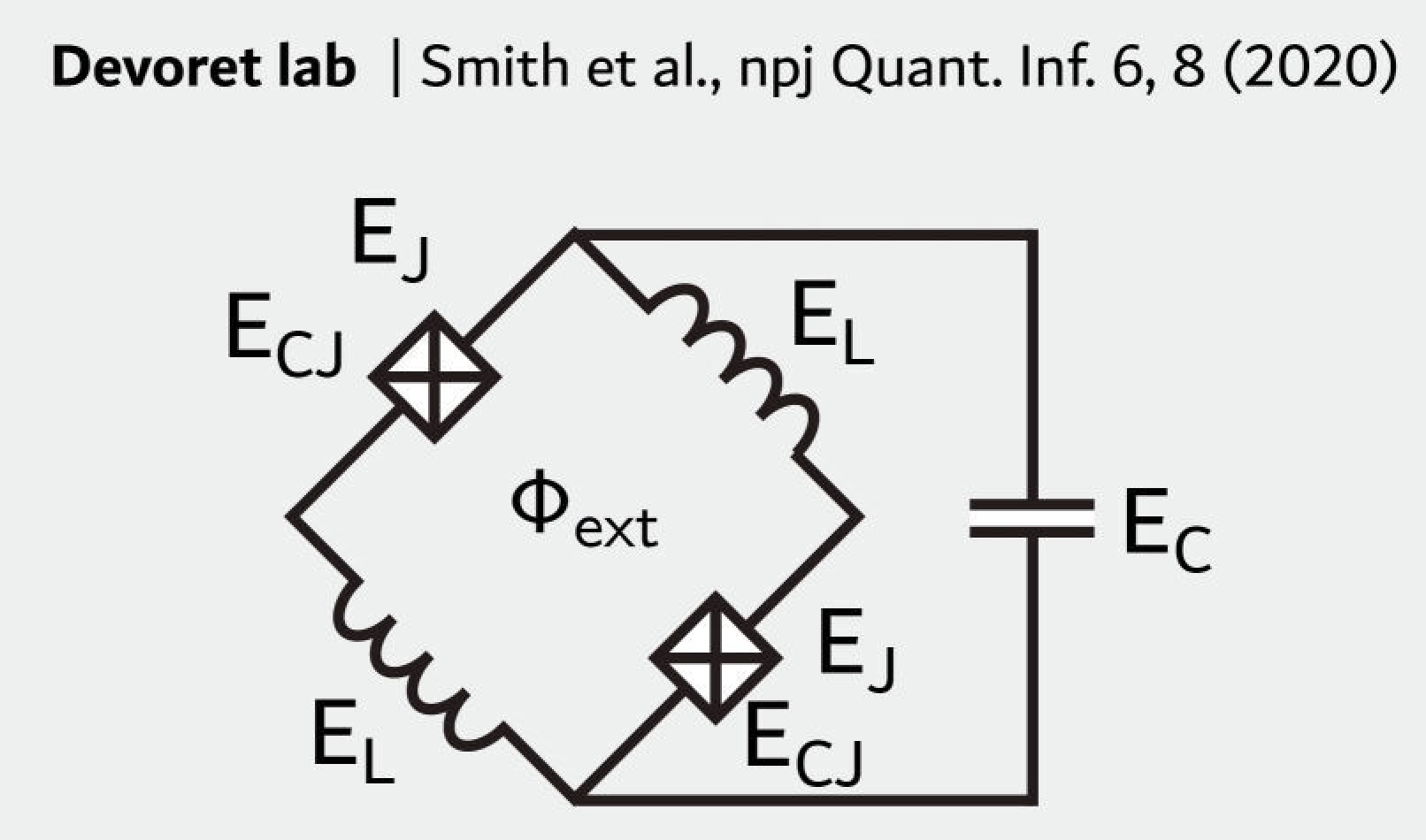
Without disorder in circuit parameters, the cos2phi qubit [Smith2020] is described by the Hamiltonian

\[\begin{split}H = & \,2 E_\text{CJ}n_\phi^2 + 2 E_\text{CJ} (n_\theta - n_\text{g} - n_\zeta)^2 + 4 E_\text{C} n_\zeta^2\\ & + E_\text{L}(\phi - \pi\Phi_\text{ext}/\Phi_0)^2 + E_\text{L} \zeta^2 - 2E_\text{J}\cos{\theta}\cos{\phi}.\end{split}\]

In the presence of disorder, the circuit is described by

\[\begin{split}H = & \,2 E_\text{CJ}'n_\phi^2 + 2 E_\text{CJ}' (n_\theta - n_\text{g} - n_\zeta)^2 + 4 E_\text{C} n_\zeta^2\\ & + E_\text{L}'(\phi - \pi\Phi_\text{ext}/\Phi_0)^2 + E_\text{L}' \zeta^2 - 2 E_\text{J}\cos{\theta}\cos{\phi} \\ & + 2 dE_\text{J} E_\text{J}\sin{\theta}\sin{\phi} \\ & - 4 dC_\text{J} E_\text{CJ}' n_\phi (n_\theta - n_\text{g}-n_\zeta) \\ & + dL E_\text{L}'(2\phi - \varphi_\text{ext})\zeta ,\end{split}\]

where \(E_\text{CJ}' = E_\text{CJ} / (1 - dC_\text{J})^2\) and \(E_\text{L}' = E_\text{L} / (1 - dL)^2\).

Here, the disorder is defined as follows: the inductive energies of the two inductors are \(E_\text{L1,2} = E_\text{L}/(1 \pm dL)\); the charging energies of the two Josephson junctions are \(E_\text{CJ1,2} = E_\text{CJ}/(1 \pm dC_\text{J})\); the junction energies of the two Josephson junctions are \(E_\text{J1,2} = E_\text{J} (1 \pm dE_\text{J})\). Alternatively, the above relations can be rewritten as: \(dL = (E_\text{L2}-E_\text{L1})/(E_\text{L2}+E_\text{L1}), E_\text{L} = 2E_\text{L1}E_\text{L2}/(E_\text{L1}+E_\text{L2})\) for inductive energies, \(dC_\text{J} = (E_\text{CJ2}-E_\text{CJ1})/(E_\text{CJ1}+E_\text{CJ2}), E_\text{CJ} = 2E_\text{CJ1}E_\text{CJ2}/(E_\text{CJ1}+E_\text{CJ2})\) for charging energies, and \(dE_\text{J} = (E_\text{J1}-E_\text{J2})/(E_\text{J1}+E_\text{J2}), E_\text{J} = (E_\text{J1}+E_\text{J2})/2\) for junction energies.

Here, we adopt notation that is consistent with other qubit classes. A conversion to the notation used in Ref. [Smith2020] can be found in the following table.

Notation used here	Notation used in Ref. [Smith2020]
\(\zeta\)	\(\theta\)
\(\theta\)	\(\varphi\)
\(\phi\)	\(\phi/2\)
\(E_\text{C}\)	\(E_\text{C} x\)
\(E_\text{CJ}\)	\(E_\text{C}\)

To numerically diagonalize the Hamiltonian of the cos2phi qubit, the harmonic basis is used for both the \(\phi\) and \(\zeta\) variables, and the charge basis is used for the \(\theta\) variable. The user needs to specify cutoffs for basis states described above, i.e., phi_cut, zeta_cut, and ncut, chosen large enough so that convergence is achieved.

An instance of the cos2phi qubit is initialized as follows:

cos2phi_qubit = scqubits.Cos2PhiQubit(EJ = 15.0,
                                      ECJ = 2.0,
                                      EL = 1.0,
                                      EC = 0.04,
                                      dCJ = 0.0,
                                      dL = 0.6,
                                      dEJ = 0.0,
                                      flux = 0.5,
                                      ng = 0.0,
                                      ncut = 7,
                                      phi_cut = 7,
                                      zeta_cut = 30)

From within Jupyter notebook, a cos2phi qubit instance can alternatively be created with:

cos2phi_qubit = scqubits.Cosi2PhiQubit.create()

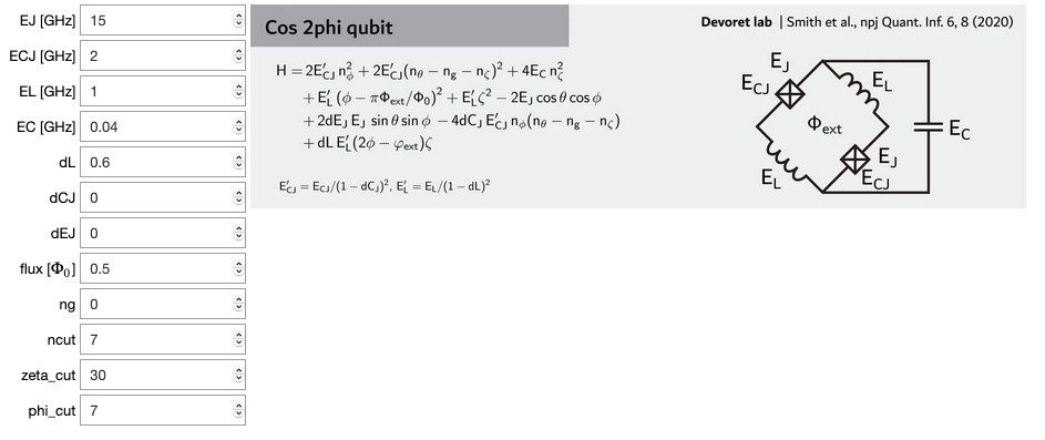
This functionality is enabled if the ipywidgets package is installed, and displays GUI forms prompting for the entry of the required parameters.

Calculational methods related to Hamiltonian and energy spectra

scqubits.Cos2PhiQubit.hamiltonian([energy_esys])	Returns Hamiltonian in basis obtained by employing harmonic basis for \(\phi, \zeta\) and charge basis for \(\theta\) or in the eigenenerg basis.
scqubits.Cos2PhiQubit.eigenvals([...])	Calculates eigenvalues using scipy.linalg.eigh, returns numpy array of eigenvalues.
scqubits.Cos2PhiQubit.eigensys([...])	Calculates eigenvalues and corresponding eigenvectors using scipy.linalg.eigh.
scqubits.Cos2PhiQubit.get_spectrum_vs_paramvals(...)	Calculates eigenvalues/eigenstates for a varying system parameter, given an array of parameter values.

Wavefunctions and visualization of eigenstates and the potential

scqubits.Cos2PhiQubit.wavefunction([esys, ...])	Return a 3D wave function in \(\phi, \zeta, \theta\) basis
scqubits.Cos2PhiQubit.plot_wavefunction([...])	Plots a 2D wave function in \(\theta, \phi\) basis, at \(\zeta = 0\)
scqubits.Cos2PhiQubit.plot_potential([...])	Draw contour plot of the potential energy in \(\theta, \phi\) basis, at \(\zeta = 0\)

Implemented operators

The following operators are implemented for use in matrix element calculations.

scqubits.Cos2PhiQubit.n_1_operator([energy_esys])	Returns operator representing the charge difference across junction 1 in native or eigenenergy basis.
scqubits.Cos2PhiQubit.n_2_operator([energy_esys])	Returns operator representing the charge difference across junction 2 in native or eigenenergy basis.
scqubits.Cos2PhiQubit.phi_1_operator([...])	Returns operator representing the phase across inductor 1 in harmonic oscillator or eigenenergy basis.
scqubits.Cos2PhiQubit.phi_2_operator([...])	Returns operator representing the phase across inductor 2 in harmonic oscillator or eigenenergy basis.
scqubits.Cos2PhiQubit.phi_operator([energy_esys])	Returns the \(\phi\) operator in the native or eigenenergy basis.
scqubits.Cos2PhiQubit.n_phi_operator([...])	Returns the \(n_\phi\) operator in the harmonic oscillator or eigenenergy basis.
scqubits.Cos2PhiQubit.n_theta_operator([...])	Returns the \(n_\theta\) operator in the charge or eigenenergy basis.
scqubits.Cos2PhiQubit.zeta_operator([...])	Returns the \(\zeta\) operator in the harmonic oscillator or eigenenergy basis.
scqubits.Cos2PhiQubit.n_zeta_operator([...])	Returns the \(n_\zeta\) operator in the harmonic oscillator or eigenenergy basis.

Computation and visualization of matrix elements

scqubits.Cos2PhiQubit.matrixelement_table(...)	Returns table of matrix elements for operator with respect to the eigenstates of the qubit.
scqubits.Cos2PhiQubit.plot_matrixelements(...)	Plots matrix elements for operator, given as a string referring to a class method that returns an operator matrix.
scqubits.Cos2PhiQubit.get_matelements_vs_paramvals(...)	Calculates matrix elements for a varying system parameter, given an array of parameter values.
scqubits.Cos2PhiQubit.plot_matelem_vs_paramvals(...)	Generates a simple plot of a set of eigenvalues as a function of one parameter.

Estimation of coherence times

scqubits.Cos2PhiQubit.plot_coherence_vs_paramvals(...)	Show plots of coherence for various channels supported by the qubit as they vary as a function of a changing parameter.
scqubits.Cos2PhiQubit.plot_t1_effective_vs_paramvals(...)	Plot effective \(T_1\) coherence time (rate) as a function of changing parameter.
scqubits.Cos2PhiQubit.plot_t2_effective_vs_paramvals(...)	Plot effective \(T_2\) coherence time (rate) as a function of changing parameter.
scqubits.Cos2PhiQubit.t1_effective([...])	Calculate the effective \(T_1\) time (or rate).
scqubits.Cos2PhiQubit.t2_effective([...])	Calculate the effective \(T_2\) time (or rate).
scqubits.Cos2PhiQubit.t1_capacitive([i, j, ...])	\(T_1\) due to dielectric dissipation in the Josephson junction capacitances.
scqubits.Cos2PhiQubit.t1_inductive([i, j, ...])	\(T_1\) due to inductive dissipation in superinductors.
scqubits.Cos2PhiQubit.t1_purcell([i, j, ...])	\(T_1\) due to dielectric dissipation in the shunt capacitor.
scqubits.Cos2PhiQubit.tphi_1_over_f(A_noise, ...)	Calculate the 1/f dephasing time (or rate) due to arbitrary noise source.
scqubits.Cos2PhiQubit.tphi_1_over_f_cc([...])	Calculate the 1/f dephasing time (or rate) due to critical current noise.
scqubits.Cos2PhiQubit.tphi_1_over_f_flux([...])	Calculate the 1/f dephasing time (or rate) due to flux noise.
scqubits.Cos2PhiQubit.tphi_1_over_f_ng([...])	Calculate the 1/f dephasing time (or rate) due to charge noise.