FluxQubit

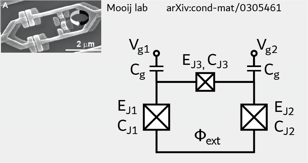
The flux qubit [Orlando1999] is described by the Hamiltonian

\[\begin{split}H_\text{flux}=&(n_{i}-n_{gi})4(E_\text{C})_{ij}(n_{j}-n_{gj}) \\ -&E_{J}\cos\phi_{1}-E_{J}\cos\phi_{2} \\ -&\alpha E_{J}\cos(2\pi f + \phi_{1} - \phi_{2}),\end{split}\]

where \(i,j \in \{1,2\}, E_\text{C}=\tfrac{e^2}{2}C^{-1}\) and

\[\begin{split}C = \left(\begin{matrix} C_{J1}+C_{g1}+C_{J3} & -C_{J3} \\ -C_{J3} & C_{J2}+C_{g2}+C_{J3} \end{matrix}\right).\end{split}\]

\(C_{Ji}\) refers to the capacitance of the \(i^\text{th}\) junction and \(C_{gi}\) refers to the capacitance to ground of the \(i^\text{th}\) island. The Hamiltonian above uses a mixed-basis notation (phase variables for the Josephson terms, charge variables for the charging energy). For numerical diagonalization, the FluxQubit class works entirely in the charge basis for both degrees of freedom. The user must specify a charge-number cutoff ncut, chosen large enough for convergence.

An instance of the flux qubit is initialized as follows. Here, the third Josephson junction is taken to be smaller than the other two by a factor \(\alpha\), the standard junction-asymmetry parameter for the three-junction flux qubit:

EJ = 35.0
alpha = 0.6
fluxqubit = scqubits.FluxQubit(EJ1 = EJ,
                              EJ2 = EJ,
                              EJ3 = alpha*EJ,
                              ECJ1 = 1.0,
                              ECJ2 = 1.0,
                              ECJ3 = 1.0/alpha,
                              ECg1 = 50.0,
                              ECg2 = 50.0,
                              ng1 = 0.0,
                              ng2 = 0.0,
                              flux = 0.5,
                              ncut = 10)

From within a Jupyter notebook, a flux qubit instance can alternatively be created with:

fluxqubit = scqubits.FluxQubit.create()

This functionality is enabled if the ipywidgets package is installed, and displays GUI forms prompting for the entry of the required parameters.

Calculational methods related to Hamiltonian and energy spectra

scqubits.FluxQubit.hamiltonian([energy_esys])	Return Hamiltonian in the basis obtained by employing charge basis for both degrees of freedom or in the eigenenergy basis.
scqubits.FluxQubit.eigenvals([evals_count, ...])	Calculates eigenvalues using scipy.linalg.eigh, returns numpy array of eigenvalues.
scqubits.FluxQubit.eigensys([evals_count, ...])	Calculates eigenvalues and corresponding eigenvectors using scipy.linalg.eigh.
scqubits.FluxQubit.get_spectrum_vs_paramvals(...)	Calculates eigenvalues/eigenstates for a varying system parameter, given an array of parameter values.

Wavefunctions and visualization of eigenstates and the potential

scqubits.FluxQubit.wavefunction([esys, ...])	Return a flux qubit wave function in \(\phi_1\), \(\phi2\) basis
scqubits.FluxQubit.plot_wavefunction([esys, ...])	Plots 2d phase-basis wave function.
scqubits.FluxQubit.plot_potential([...])	Draw contour plot of the potential energy.

Implemented operators

The following operators are implemented for use in matrix element calculations.

scqubits.FluxQubit.n_1_operator([energy_esys])	Returns the charge number operator conjugate to \(\phi_1\) in the charge? or eigenenergy basis.
scqubits.FluxQubit.n_2_operator([energy_esys])	Returns the charge number operator conjugate to \(\phi_2\) in the charge? or eigenenergy basis.
scqubits.FluxQubit.exp_i_phi_1_operator([...])	Returns operator \(e^{i\phi_1}\) in the charge or eigenenergy basis.
scqubits.FluxQubit.exp_i_phi_2_operator([...])	Returns operator \(e^{i\phi_2}\) in the charge or eigenenergy basis.
scqubits.FluxQubit.cos_phi_1_operator([...])	Returns operator \(\cos \phi_1\) in the charge or eigenenergy basis.
scqubits.FluxQubit.cos_phi_2_operator([...])	Returns operator \(\cos \phi_2\) in the charge or eigenenergy basis.
scqubits.FluxQubit.sin_phi_1_operator([...])	Returns operator \(\sin \phi_1\) in the charge or eigenenergy basis.
scqubits.FluxQubit.sin_phi_2_operator([...])	Returns operator \(\sin \phi_2\) in the charge or eigenenergy basis.

Computation and visualization of matrix elements

scqubits.FluxQubit.matrixelement_table(operator)	Returns table of matrix elements for operator with respect to the eigenstates of the qubit.
scqubits.FluxQubit.plot_matrixelements(operator)	Plots matrix elements for operator, given as a string referring to a class method that returns an operator matrix.
scqubits.FluxQubit.get_matelements_vs_paramvals(...)	Calculates matrix elements for a varying system parameter, given an array of parameter values.
scqubits.FluxQubit.plot_matelem_vs_paramvals(...)	Generates a simple plot of a set of eigenvalues as a function of one parameter.

Estimation of coherence times

scqubits.FluxQubit.plot_coherence_vs_paramvals(...)	Show plots of coherence for various channels supported by the qubit as they vary as a function of a changing parameter.
scqubits.FluxQubit.plot_t1_effective_vs_paramvals(...)	Plot effective \(T_1\) coherence time (rate) as a function of changing parameter.
scqubits.FluxQubit.plot_t2_effective_vs_paramvals(...)	Plot effective \(T_2\) coherence time (rate) as a function of changing parameter.
scqubits.FluxQubit.t1(i, j, noise_op, ...[, ...])	Calculate the transition time (or rate) using Fermi's Golden Rule due to a noise channel with a spectral density spectral_density and system noise operator noise_op.
scqubits.FluxQubit.t1_effective([...])	Calculate the effective \(T_1\) time (or rate).
scqubits.FluxQubit.t2_effective([...])	Calculate the effective \(T_2\) time (or rate).
scqubits.FluxQubit.tphi_1_over_f(A_noise, i, ...)	Calculate the 1/f dephasing time (or rate) due to arbitrary noise source.
scqubits.FluxQubit.tphi_1_over_f_cc([...])	Calculate the 1/f dephasing time (or rate) due to critical-current noise from all three Josephson junctions \(EJ1\), \(EJ2\) and \(EJ3\).