ZeroPi#

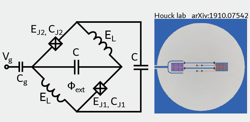
The Zero-Pi qubit [Brooks2013] [Dempster2014], when decoupled from the zeta mode, is described by the Hamiltonian

\[\begin{split}H &= -2E_\text{CJ}\partial_\phi^2+2E_{\text{C}\Sigma}(i\partial_\theta-n_g)^2 +2E_{C\Sigma}dC_J\,\partial_\phi\partial_\theta\\ &\qquad -2E_\text{J}\cos\theta\cos(\phi-\varphi_\text{ext}/2)+E_L\phi^2+2E_\text{J} + E_J dE_J \sin\theta\sin(\phi-\varphi_\text{ext}/2)\end{split}\]

expressed in phase basis. The definition of the relevant charging energies \(E_\text{CJ}\), \(E_{\text{C}\Sigma}\), Josephson energies \(E_\text{J}\), inductive energies \(E_\text{L}\), and relative amounts of disorder \(dC_\text{J}\), \(dE_\text{J}\) follows [Groszkowski2018].

Internally, the ZeroPi class formulates the Hamiltonian matrix by discretizing the phi variable, and using charge basis for the theta variable.

An instance of the Zero-Pi qubit is created as follows:

phi_grid = scqubits.Grid1d(-6*np.pi, 6*np.pi, 200)

zero_pi = scqubits.ZeroPi(grid = phi_grid,
                           EJ   = 0.25,
                           EL   = 10.0**(-2),
                           ECJ  = 0.5,
                           EC   = None,
                           ECS  = 10.0**(-3),
                           ng   = 0.1,
                           flux = 0.23,
                           ncut = 30)

Here, flux is given in units of the flux quantum, i.e., in the form \(\Phi_\text{ext}/\Phi_0\). In the above example, the disorder parameters dEJ and dCJ are not specified, and hence take on the default value zero (no disorder).

From within Jupyter notebook, a fluxonium instance can alternatively be created with:

zero_pi = scqubits.ZeroPi.create()

This functionality is enabled if the ipywidgets package is installed, and displays GUI forms prompting for the entry of the required parameters.

Wavefunctions and visualization of eigenstates#

`scqubits.ZeroPi.wavefunction`([esys, which, ...])	Returns a zero-pi wave function in phi, theta basis
`scqubits.ZeroPi.plot_wavefunction`([esys, ...])	Plots 2d phase-basis wave function.

Implemented operators#

The following operators are implemented for use in matrix element calculations.

`scqubits.ZeroPi.i_d_dphi_operator`()	Operator \(i d/d\phi\).
`scqubits.ZeroPi.phi_operator`([energy_esys])	Returns \(\phi\) operator in the native or eigenenergy basis.
`scqubits.ZeroPi.n_theta_operator`([energy_esys])	Returns \(n_\theta\) operator in the native or eigenenergy basis.
`scqubits.ZeroPi.cos_theta_operator`([energy_esys])	Returns \(\cos(\theta)\) operator in the native or eigenenergy basis.
`scqubits.ZeroPi.sin_theta_operator`([energy_esys])	Returns \(\sin(\theta)\) operator in the native or eigenenergy basis.

Computation and visualization of matrix elements#

`scqubits.ZeroPi.matrixelement_table`(operator)	Returns table of matrix elements for operator with respect to the eigenstates of the qubit.
`scqubits.ZeroPi.plot_matrixelements`(operator)	Plots matrix elements for operator, given as a string referring to a class method that returns an operator matrix.
`scqubits.ZeroPi.get_matelements_vs_paramvals`(...)	Calculates matrix elements for a varying system parameter, given an array of parameter values.
`scqubits.ZeroPi.plot_matelem_vs_paramvals`(...)	Generates a simple plot of a set of eigenvalues as a function of one parameter.

Utility method for setting charging energies#

scqubits.ZeroPi.set_EC_via_ECS(ECS)

Helper function to set EC by providing ECS, keeping ECJ constant.

Estimation of coherence times#

`scqubits.ZeroPi.plot_coherence_vs_paramvals`(...)	Show plots of coherence for various channels supported by the qubit as they vary as a function of a changing parameter.
`scqubits.ZeroPi.plot_t1_effective_vs_paramvals`(...)	Plot effective \(T_1\) coherence time (rate) as a function of changing parameter.
`scqubits.ZeroPi.plot_t2_effective_vs_paramvals`(...)	Plot effective \(T_2\) coherence time (rate) as a function of changing parameter.
`scqubits.ZeroPi.t1`(i, j, noise_op, ...[, T, ...])	Calculate the transition time (or rate) using Fermi's Golden Rule due to a noise channel with a spectral density spectral_density and system noise operator noise_op.
`scqubits.ZeroPi.t1_effective`([...])	Calculate the effective \(T_1\) time (or rate).
`scqubits.ZeroPi.t1_flux_bias_line`([i, j, M, ...])	Noise due to a bias flux line.
`scqubits.ZeroPi.t1_inductive`([i, j, Q_ind, ...])	\(T_1\) due to inductive dissipation in a superinductor.
`scqubits.ZeroPi.t2_effective`([...])	Calculate the effective \(T_2\) time (or rate).
`scqubits.ZeroPi.tphi_1_over_f`(A_noise, i, j, ...)	Calculate the 1/f dephasing time (or rate) due to arbitrary noise source.
`scqubits.ZeroPi.tphi_1_over_f_cc`([A_noise, ...])	Calculate the 1/f dephasing time (or rate) due to critical current noise.
`scqubits.ZeroPi.tphi_1_over_f_flux`([...])	Calculate the 1/f dephasing time (or rate) due to flux noise.

`scqubits.ZeroPi.hamiltonian`([energy_esys])	Calculates Hamiltonian in basis obtained by discretizing \(\phi\) and employing charge basis for \(\theta\) or in the eigenenergy basis.
`scqubits.ZeroPi.eigenvals`([evals_count, ...])	Calculates eigenvalues using scipy.linalg.eigh, returns numpy array of eigenvalues.
`scqubits.ZeroPi.eigensys`([evals_count, ...])	Calculates eigenvalues and corresponding eigenvectors using scipy.linalg.eigh.
`scqubits.ZeroPi.get_spectrum_vs_paramvals`(...)	Calculates eigenvalues/eigenstates for a varying system parameter, given an array of parameter values.